LSTMs or Long Short-Term Memory Networks have been around for a long time. They have been applied for quite a few sequence-related tasks such as text generation and translation or even generating image captions.

Their drawback has been that they couldn’t be parallelized to make use of the powerful modern-day GPUs. This limitation paved the way for the emergence of transformers that leverage GPUs for massive parallelization of training and inference.

If we now make an attempt to revamp and parallelize LSTMs, can the LSTMs become the tool to build next-generation LLMs?

This is the exact question answered by the paper “XLSM — Extended Long Short-term Memory Networks” which stands for “extended” Long short-term memory. They do so by proposing two novel blocks in the architecture namely, sLSTM and mLSTM.

So let's dive deep into the proposed sLSTM and mLSTM blocks proposed in this paper and see how we can stack them together to develop the XLSTM architecture.

Visual Explanation

If you are someone like me and would like XLSTMs explained visually, then please check the YouTube video on this article:

LSTM refresher

One of the earliest networks designed to tackle sequential data is the Recurrent Neural Network.

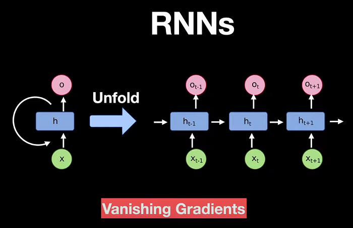
It uses recurrent connections in its architecture with x as input and o as output. If we unfold it, we can visualize it as a sequence of operations happening at time stamps, t-1, t, and t+1. A major drawback of RNNs was the vanishing gradient problem where the gradient gets to zero as we stack too many blocks together.

LSTMs or Long short-term memory networks were proposed to overcome the vanishing gradients by introducing cell states and gating mechanism to the network.

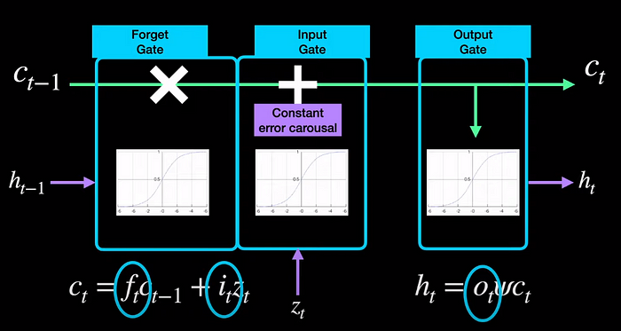
The cell states, c, are long-term memories that live across several time stamps. The hidden states, h, are short-term memories that are passed along from one time step to another. And of course, we have the inputs, z, from the input sequence.

Three gates have S-shaped functions. The forget gate uses a sigmoid function to decide what information to forget in long-term memory. The input gate also uses a sigmoid function to process the input and adds it to the output of the forget gate. This addition operation has a fancy term called constant error carousal in the XLSTM paper and the academic literature. This addition operation is what tackles the vanishing gradients problem found in RNNs. The output c_t is then processed by the output gate which usually is a tanh function leading to the hidden state output h_t that is passed on to the next time step.

With these operations, we have dissected the two main equations of LSTMs which are that of c_t and h_t.

Drawback 1 — Revising Storage Decisions

One of the main drawbacks of LSTMs is their inability to revise storage decisions. What it means is that as the sequence length increases, the model should be able to decide whether it keeps past information or not in the memory.

For example, if we take this sentence, “Tom went to the shop. He bought some drinks” and compare it with “Tom went to the shop to buy some groceries which included carrots, onions, bananas, apples, oranges, coffee and bread. He also bought some drinks.” For every new word such as bananas or apples, the model has to constantly revise whether it should hold the past word “Tom” in its memory. This is a big challenge to the LSTMs and it stems from the sigmoid function in its forget gate.

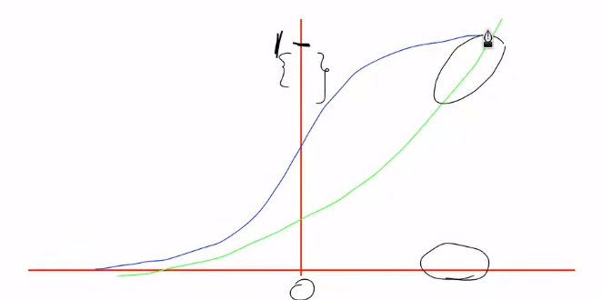
So if we take a forget gate, it is composed of a sigmoid function which has an S-shaped curve that flattens towards the end. This indicates that as we move towards the higher values of input, the decision as to what to forget and what to keep in the memory becomes quite challenging. But if we use an exponential function in its place, then the game changes, and as we go to higher values of the input, we get a wider range for the outputs. This in turn indicates that LSTMs can get better at revising storage decisions.

Solution 1 — sLSTM

So the solution proposed in this paper is the sLSTM blocks. If we go back to the classic LSTM equation that represents the cell state, as we saw before, it is a function of the forget gate and the input gates.

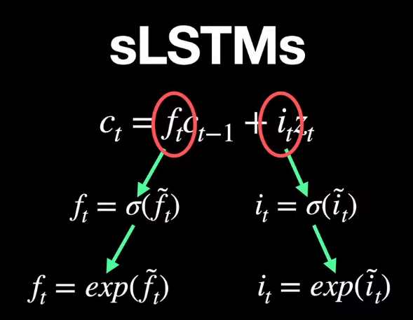
These gates in turn are composed of sigmoid functions. So, what if we replace these sigmoid functions with exponential functions? The new gates f_t and i_t now become exp(f_t) and exp(i_t) and that pretty much is the main modification to create the sLSTM block.

Unlike the sigmoid function which squeezes the inputs to be in a fixed range, the exponential functions tend to blow up in value as the input increases and it does not naturally normalize the output to lie between say, 0 and 1 like the sigmoid function.

So, we need to introduce a new normalizer state which is a function of the forget and input gates. We can think of it as a running average of a normalization value.

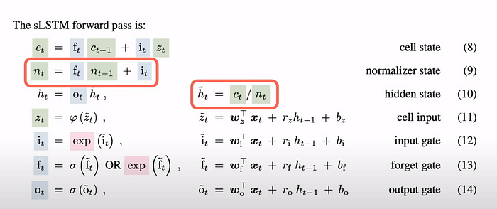
We use the calculated normalization values to normalize the output or the new hidden state.

While the normalization takes care of the hidden states, to control the exponential from blowing up the forget and input gates, we need to introduce a stabilizer. It comes in the form of log functions to counter the effect of the exponentials and introduce stability. So the stabilizer state is the max of the log of the forget gate and input gate output. We subtract these stabilizer values from the input and forget gates to stabilize them

Drawback 2 — Memory and Parallelization

The second drawback of the LSTMs is the lack of parallelization. The LSTMs were designed to handle sequential data which means it needs the output of processing the previous input in the sequence to process the current input in the sequence. This particular drawback prevents parallelization and was the culprit that led to the dawn of the Transformers era.

The solution proposed in this paper is the novel mLSTM blocks. So, let's look at them next.

Solution 2 — mLSTM

The next building block of XLSTMs is the mLSTM block where m stands for memory. Let's go back to the classic LSTM equation again to see what the drawback of it is. we can see that the cell state c_t is a scalar. This means we only deal with 1 number at a time when we have the luxury of modern-day GPUs with at least 12 Gigs of memory.

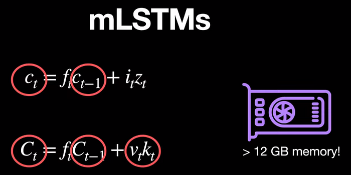
The mLSTM block introduces matrices in place of scalars for the cell states. Going back to our classic equation of LSTM, What if we replace the c_t with a matrix C_t so the cell state now becomes capital C_t to indicate matrices and the cell states can be retrieved not just by a gate i_t but by storing key-value pairs which are vectors. The values of which can be retrieved by queries which are vectors of the same dimension.

To make it sound familiar to the transformer terminology, they have introduced key and value here to form this matrix.

XLSTM

With that information on the sLSTM and mLSTM, let's dive into the detailed architecture of XLSTM.

sLSTM

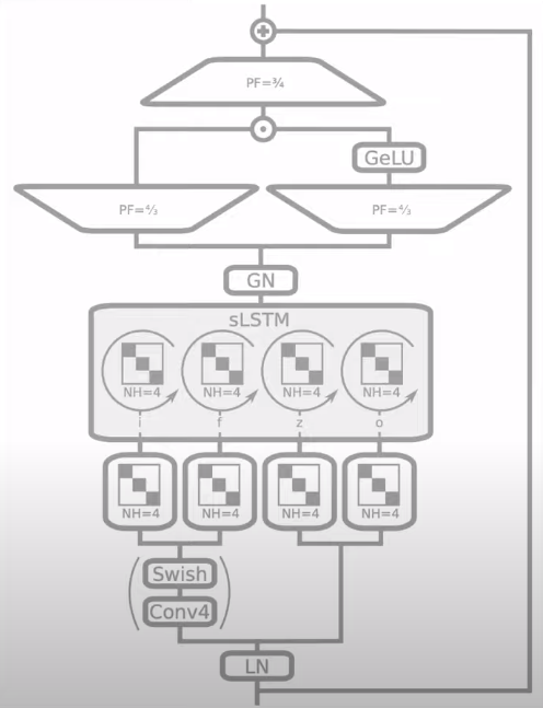
When it comes to sLSTM, we use post-up projections. So the input is first passed through causal convolution layers with a swish activation function. The output from these layers is then fed through a block-diagonal linear layer with four diagonal blocks or “heads”. The output from these is then fed through the sLSTM block with 4 heads. Finally, the output is up-projected using a gated MLP layer with GeLU activation and down-projected using a gated MLP function.

mLSTM

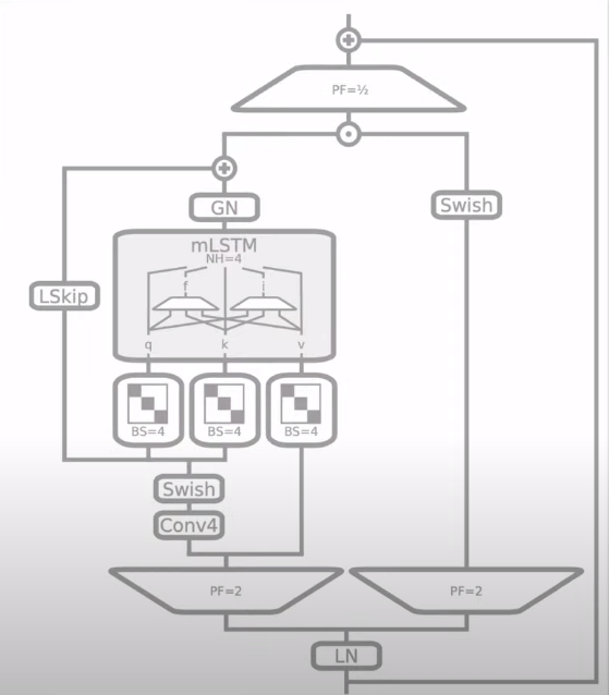
Moving on to the details of the mLSTM block, we use pre-up projections. Meaning that the input is first up-projected with a projection factor of 2. One of the projection outputs goes to the mLSTM and another goes to the output gate. The input to the mLSTM block goes through causal convolution and then through block diagonal projection matrices of block size 4 which output the query, key, and value that is readily used by the mLSTM block.

XLSTM Architecture

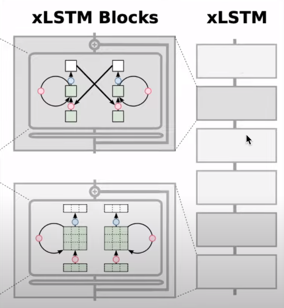
Finally, we can then stack the two types of blocks to form the extended LSTM architecture. So the dark grey blocks are the mLSTM blocks and the light grey ones are the sLSTM blocks.

In terms of the advantages, the paper mentions that the XLSTM networks have a linear computational complexity and a constant memory complexity concerning the sequence length.

Evaluations

The authors have trained on the SlimPajama dataset to compare against other transformer-based methods like LLAMA and state-space based methods like MAMBA. They have used this notation of xLSTM a:b where a is the number of mLSTM blocks and b is the number of sLSTM blocks in the stack.

In terms of the accuracies, they report relative accuracies by scaling accuracies between 0 and 1 where 0 is random and 1 is perfect.

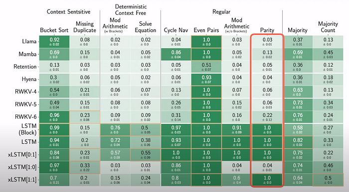
From the results, something that is of particular interest is the parity task where the transformers or the state-space models tend to struggle without memory mixing or state tracking. We can see that in this kind of task, the xLSTM hits an accuracy of 1 when we use both the sLSTM and mLSTM blocks together.

They have also done some ablation studies to show the robustness of XLSTMs. They are easy to understand from the paper. Moreover, this article is more about the architectural novelties of XLSTMs so I am not going into the experimental results here.

Shout Out

If you liked this article, why not follow me on Twitter where I share research updates from top AI labs every single day of the week?

Also please subscribe to my YouTube channel where I explain AI concepts and papers visually.

Conclusion

Hope this article simplified and eased the understanding of the XLSTM architecture, why we need them, and how they could potentially overtake transformers in the near future.

Let's wait and see what they have in store. I will see you in my next…