RAG - 7 indexing methods for Vector DBs + Similarity search

In my previous articles, we saw about data ingestion into a RAG pipeline. We then saw about BERT and SBERT which are the most popular embedding models for RAGs. The next step of embedding the inputs is storing the embeddings in a persistent store. Storing the embeddings saves computational overhead if we want to use the embeddings repeatedly.

Though there are numerous types of databases like relational, NoSQL, and Graph DBs, the go-to choice for a RAG pipeline is Vector DBs. This is because Vector DBs support horizontal scaling and metadata filtering on top of the CRUD operation, which is commonly available in other databases. 

In this post, let's dive deep into Vector DBs and understand their components, strengths and weaknesses thoroughly. 

Why Vector DBs

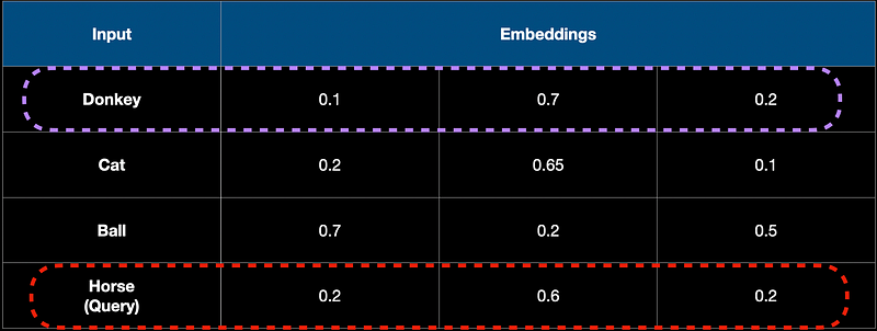
Let's say we have 1000 documents in our RAG system. We have chunked and embedded them into vectors. Let the vectors be of dimension 3 in this toy scenario and let's say we have 3 words in the DB which are dog, cat, and ball. We choose to store the embeddings in a traditional, relational DB in a table say, embeddings. Let the user query for the horse when interacting with the RAG/LLM system. 

A relational DB searches for the exact match for a query. A vector DB on the other hand retrieves the “most similar” record from the DB. To achieve this they do something called the Approximate Nearest Neighbour Search (ANN) search. ANN works by finding the most similar item (in meaning) from the DB rather than finding the exact match for the query. For example, if the user queries for “Horse”, a relational DB without an entry for “Horse” will not return anything. But a Vector DB would return “Donkey” as it is semantically similar to a Horse.

Vector DBs vs Others

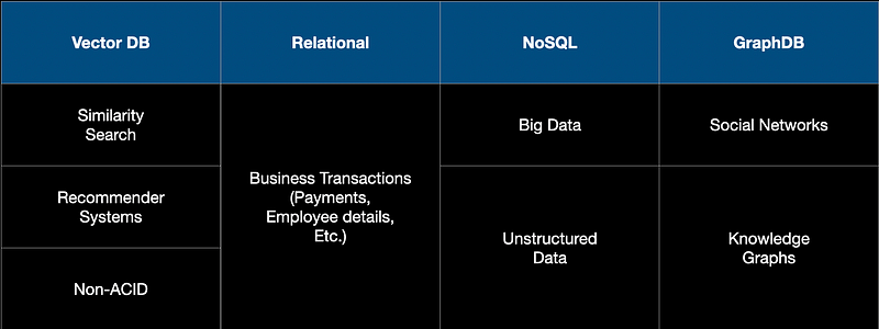
Just to get the big picture, let's briefly look at the type of DBs available today. The different types are shown in the table below. Each DB is designed for a special purpose. As an example, relational DBs are mainly transactions and use structured tables. We are all quite familiar with them as these are the oldest technology of all. Then came NoSQL DBs like Mongo DB that are designed for unstructured data like documents, images, and really long text. Graph DBs slowly emerged alongside the social media revolution that took place in the 2000s. A good example of this would be Neo4J DB.

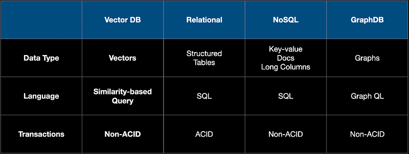
In terms of the applications, relational DBs are used for applications such as banking, insurance, and HR for say, tracking employee records in a HR system. While NoSQL DBs like Mongo DB are used to store massive documents, images, and long text files. Graph DBs like Neo4J are used to store data that tend to have graphical relationships. For example, if we are designing a social network site, then the relationship between people can be better captured with a graph DB. 

So, How do Vector DBs work?

Unlike relational or NoSQL DBs that store scalar data in rows and columns, vector DBs store vectors. The vectors are high dimensional and are the result of the embedding models used in AI systems today. So, Vector DBs are optimized for storing and querying these vectors.

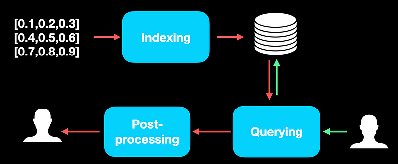
The main steps in designing and maintaining a Vector DB are indexing, querying, and a possible post-processing step once the needed records are retrieved from the vector DB. 

Let's look into each of these steps.

Indexing

Indexing is the most crucial part of a Vector DB. The whole purpose of storing the embeddings in a DB is to retrieve them seamlessly and indexing plays a crucial role in this process. So, we need efficient algorithms for indexing and specific use cases. Below are some common algorithms used for indexing:

Flat Indexing or Exact Match

Flat indexing is a brute-force algorithm. Here we do not modify the input vectors, nor do we cluster them. Whenever we get a new query point, we compare it against all the other full-sized vectors in our index and calculate the distances. We then return the closest k vectors, where k is a pre-defined hyperparameter. 

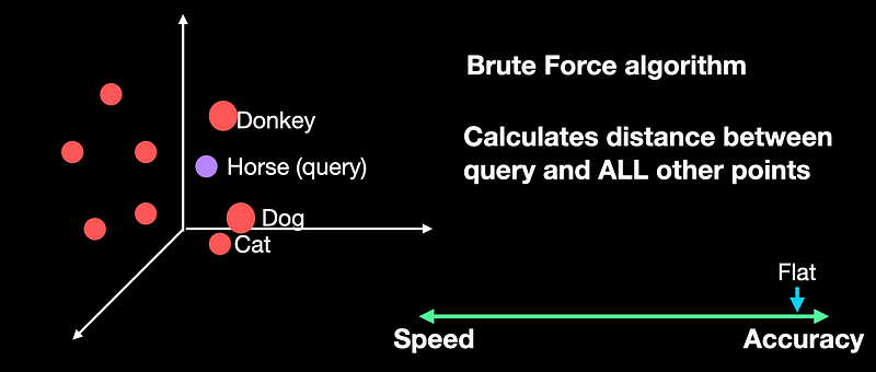
Flat index does no approximation of the vectors. It compares the query against every other vector in the DB, it's the most accurate of all indexing algorithms. But in the accuracy-speed trade-off, it tends to be the slowest as it's a brute-force algorithm.

There are two ways in which we can reduce the speed of search: 

• Reduce the vector size (dimensions). We can reduce the dimension of vectors from say 128 to 64 and hence all the associated computation.
• Reduce the search scope. In a DB of 100 vectors, what if we search only 60 and ignore the rest?

So, below are some of the algorithms that adapt one of the above approaches to reduce computation at the cost of accuracy or memory.

Local Sensitivity Hashing

What if we have millions of documents with a few duplicates and a few that are quite similar? It works by grouping high-dimensional vectors into different buckets. They use hashing functions for grouping. 

These are the steps we follow:

1. We first convert the input documents into shingles with a fixed k. For example, if our input word is, “AI Bites” and k = 2, then the shingles will be “AI”, “Bi”, “it”, “te”, “es”. 
2. As there will be too many shingles per document, we then convert the shingles into 1-hot encodings using a fixed vocabulary for the dataset. 
3. Convert the 1-hot encodings into signatures using the MinHashing algorithm. 
4. The hashed signatures are then mapped into hashing buckets using some hashing functions. 

The most tricky bit is understanding the MinHasing algorithm. I have given a simple example below so that it's easier to grasp. I have shown 2 random permutations and two documents converted into 1-hot encodings. Each permutation forms a row in the signature. For each permutation, we start with 1 and check if the document has a 1-hot encoding value of 1. If yes, then we enter the value of permutation as the signature. We do this for all permutation+document combinations. 

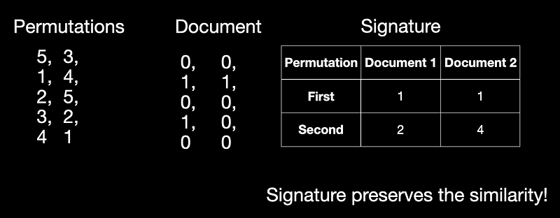
Building this signature has significantly reduced the memory but preserves the similarities at the same time. Whenever we get a new query vector, it is sufficient to search inside a single bucket, ignoring the rest. 

The performance of LSH depends on the hashing function and the size and number of buckets used. These hash tables grow large with data and they need to be stored which is an overhead for LSH. It is designed for large, high-dimensional datasets. It provides significant speed-up compared to the flat index. 

Hierarchical Navigable Small World(HNSW)]

HNSW is a graph-based algorithm. To understand HNSW, let’s start with NSW and create a data structure which is a graph. Given a bunch of documents, we start with the first and incrementally build a graph by adding one additional document at a time. 

To build the graph, let’s fix a value of k as say 2 for this. We start with one node and keep adding nodes one at a time. If the similarity of the new node is lower than the first, we link it. Otherwise, we ignore it. 

To query, let’s say we have a graph with 6 documents. We start with a random node. We traverse to the next node if the similarity is smaller than the current similarity. We do so until we reach the last node where none of its neighbors have a lower similarity. 

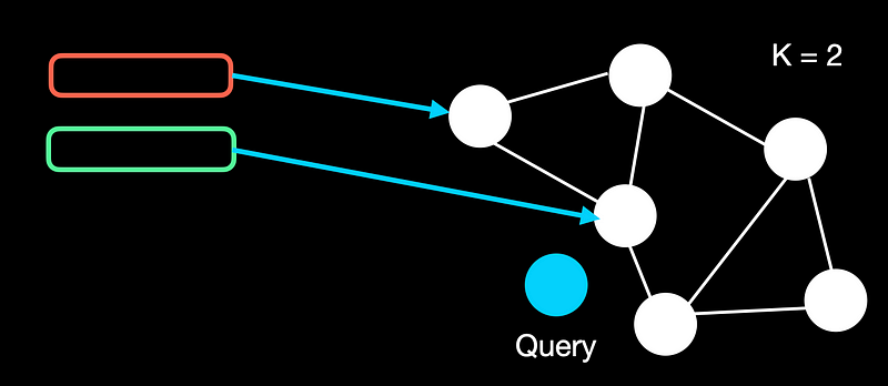
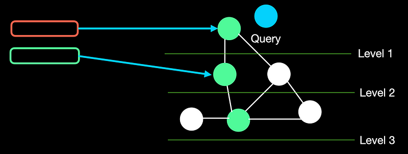
HNSW advances NSW and creates a tree-like hierarchical structure by grouping a set of nodes into a layer. The nodes are connected by edges which represent their similarity. 

Whenever HNSW gets a query, the algorithm starts with a random node in the highest layer. If a node at the next lower level has higher similarity, it traverses 1 level lower. We stop when we hit the last layer and none of the nodes has a better similarity score. We then return the top-k nodes from the traversal path. 

Inverted File (IVF) Indexing

IVF is a clustering-based algorithm. It’s a very popular index as it’s easy to use, has high search quality, and has reasonable search speed. 

It works on the concept of Voronoi diagrams, also called Dirichlet tessellation. To understand it, let's imagine our highly-dimensional vectors placed into a 2D space. We then place a few additional points in our 2D space, which will become our ‘cluster’ (Voronoi cells in our case) centroids.

We then extend an equal radius out from each of our centroids. At some point, the circumferences of each cell circle will collide with another — creating our cell edges:

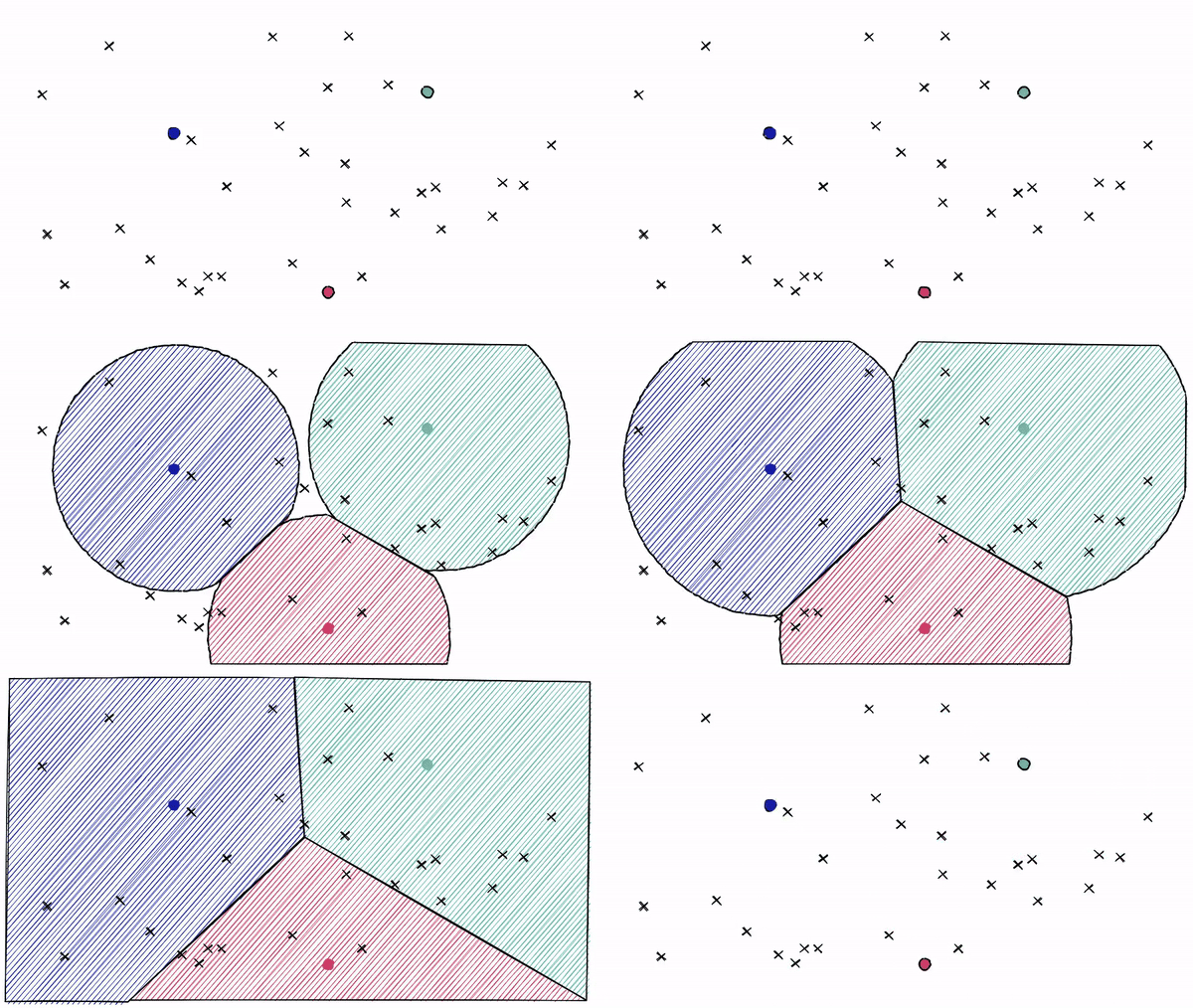
But what if a data point falls at the boundary between two cells? This is called the edge problem. To overcome this, the algorithm proposes something called the probes. Probes are just the number of cells we will inspect. For example, if nprobles = 8, we will inspect 8 cells rather than just one as shown in the figure below.

Product Quantization

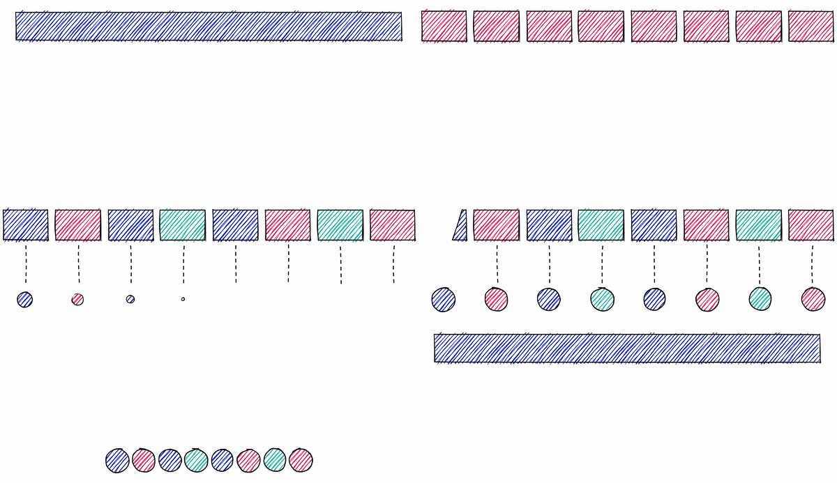
The idea of PQ is extremely simple. It effectively works by following the below steps:

• Split the long input vectors into equal-sized sub-vectors or partitions
• We treat each partition separately and cluster them using k-means to create a centroid for each group. The centroids are stored and act as representatives for the vectors it contain. 
• Whenever we have a query vector, we partition it. We compare the partitions with the centroids in each group. We identify the closest centroid and return partitions belonging to that cluster.

Approximate Nearest Neighbour Oh Yeah(ANNOY)

Annoy is a C++ library designed by Spotify and it has a Python binding. It is designed for efficiency and simplicity to spot data points in space that are closest to a given data/query point. 

In the indexing phase, Annoy starts by partitioning the given data into halves. It keeps partitioning the vectors until there is a max of k vectors in each of the partitions. k is usually about 100, but it also depends on the data on hand.

During the query phase, we start at the top of the hierarchy and traverse based on which leaf node is closest to the query. After traversing to the leaf node, we have an array of vectors that are similar to the query. The k nodes that fall within that partition are now returned as response to the query.

Random Projection

The basic idea behind random projection is to project the high-dimensional vectors to a lower-dimensional space using a random projection matrix. We follow the below steps:

• Create a matrix of random numbers. The size of the matrix is going to be the target low-dimension value we want. 
• Calculate the product of the input vectors and the matrix, which results in a projected matrix that has fewer dimensions than our original vectors but still preserves their similarity.
• When we get a query, we use the same random projection matrix to project the query. As similarity is preserved in the lower dimensional space, the same vectors should be returned both in the high and low dimensional space

Querying and Similarity metrics

Similarity measures define how the database identifies results for a user query. These are well-established mathematical approaches in machine learning. The most common similarity measures are:

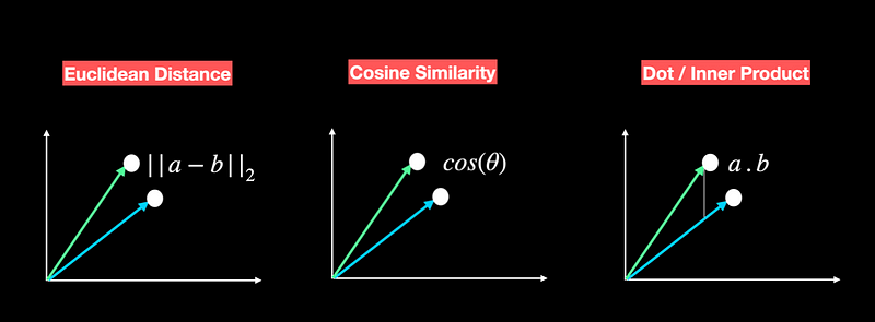
• Dot Product. measures the product of the magnitudes of two vectors and the cosine of the angle between them. A positive value represents vectors that point in the same direction (angle less than 90 degrees), 0 represents orthogonal vectors, and a negative value represents vectors that are at an angle greater than 90 degrees.
• Cosine Similarity. It measures the cosine of the angle between two vectors in a vector space. It ranges from -1 to 1, where 1 represents identical vectors, 0 represents orthogonal vectors, and -1 represents vectors that are diametrically opposed.
• Euclidean Distance measures the straight-line distance between two vectors in a vector space. It ranges from 0 to infinity, where 0 represents identical vectors, and larger values represent increasingly dissimilar vectors.

Conclusion

To summarize, we saw an overview of Vector DBs and understood why we need them in the first place. We also saw 7 indexing algorithms that are used to speed up querying Vector DBs and making them super efficient. We do all the indexing to query similar records in the DB. 

In the coming weeks, let's look into the concepts in RAG before moving on to advanced RAG and some hands-on RAG pipeline development. Till then, please stay tuned…