Model Quantization in Deep Learning

Quantization in general can be defined as mapping values from a large set of real numbers to values in a small discrete set . Typically this involves mapping continuous inputs to fixed values at the output. A common way we can think of achieving this is by rounding or truncating. In case of rounding, we compute the nearest integer. For example, a value of 1.8 becomes 2. But a value of 1.2 becomes 1. In case of truncation, we blindly remove the values after the decimal to convert the input to an integer.
Motivation for Quantization
In whichever way we proceed, the main motivation behind quantization of deep neural networks is to improve the inference speed as its needless to say that inference and training of NNs is computationally quite expensive. With the advent of Large Language Models, the number of parameters in these models are only increasing meaning that the memory footprint is only getting higher and higher. With the speed at which these neural networks are evolving, there is increasing demand to run these neural networks on our laptops or mobile phones and even tiny devices like watches. None of this is possible without quantization.
Before diving into quantization, lets not forget that trained Neural Networks are mere floating numbers stored in computer’s memory.


Some of the well known representations or formats for storing numbers in computers are float32 or FP32, float16 or FP16 , int8, bfloat16 B stands for Google Brain or more recently, tenfor float 32, a specialised format for handling matrix or tensor operations. Each of these formats consume different chunk of the memory.
For example, float32 allocates 1 bit for sign, 8 bits for exponent and 23 bits for mantissa.
Similarly, float16 or FP16 allocates 1 bit for sign but just 5 bits for exponent and 10 bits for mantissa. On the other hand, BF16 allocates 8 bits for the exponent and just 7 bits for mantissa.
Quantization in deep networks
Enough on representations. What I mean to say is, the conversion from a higher memory format to a lower memory format is called quantization. Talking in deep learning terms, Float32 is referred to as single or full precision and Float16 and BFloat16 are called half precision. The default way in which deep learning models are trained and stored is in full precision. The most commonly used conversion is from full precision to an int8 format.
Types of Quantization
Quantization can be uniform or non-uniform. In the uniform case, the mapping from the input to the output is a linear function resulting in uniformly spaced outputs for uniformly spaced inputs. In the non-uniform case, the mapping from the input to the output is a non-linear function and so the outputs won’t be uniformly spaced for an uniform input.
Diving into the uniform type, the linear mapping function can be a scaling and rounding operation . And so uniform quantization involves a scaling factor, S in the equation.
When converting from say float16 to int8, notice that we can always restrict to values between -127 and plus 127 and ensure that the zero of the input perfectly maps to the zero of the output leading to a symmetric mapping and this quantization is therefore called symmetric quantization.
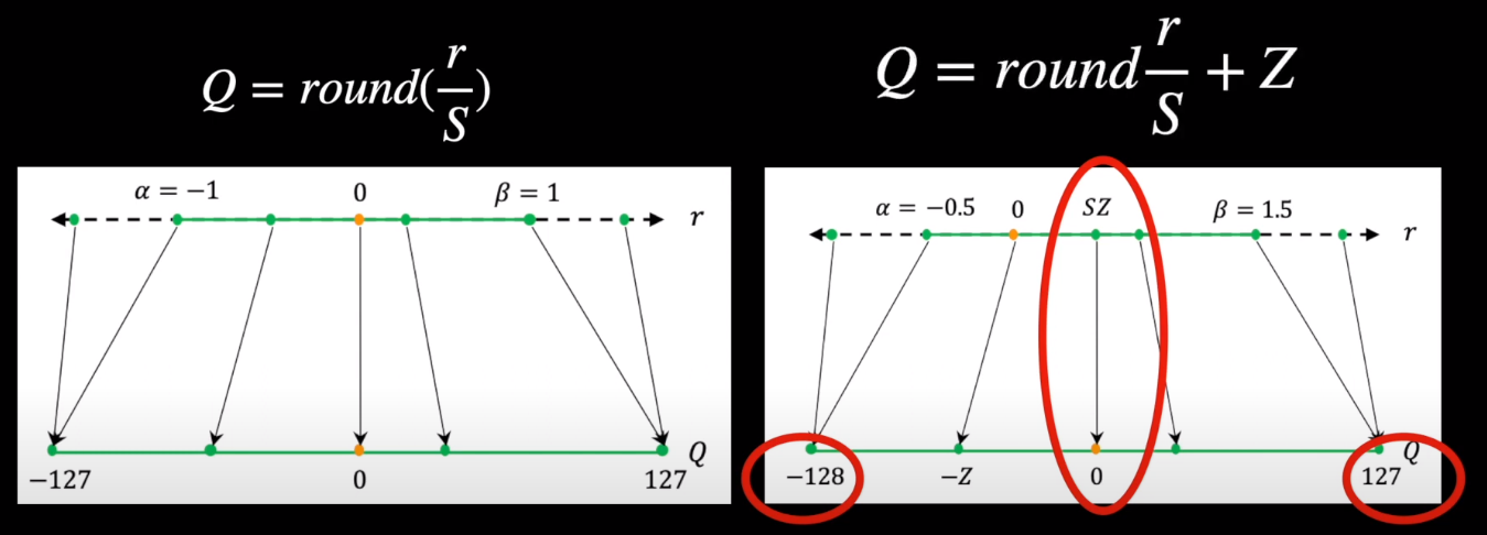
On the other hand, if the values on either side of zero are not the same for example between -128 and +127. And additionally if we are mapping the zero of the input to some other value other than zero at the output , then its called asymmetric quantization. As we now have the zero value shifted in the output, we need to count for this in our equation by including the zero factor, Z, in the equation.
Choosing Scale and zero factor
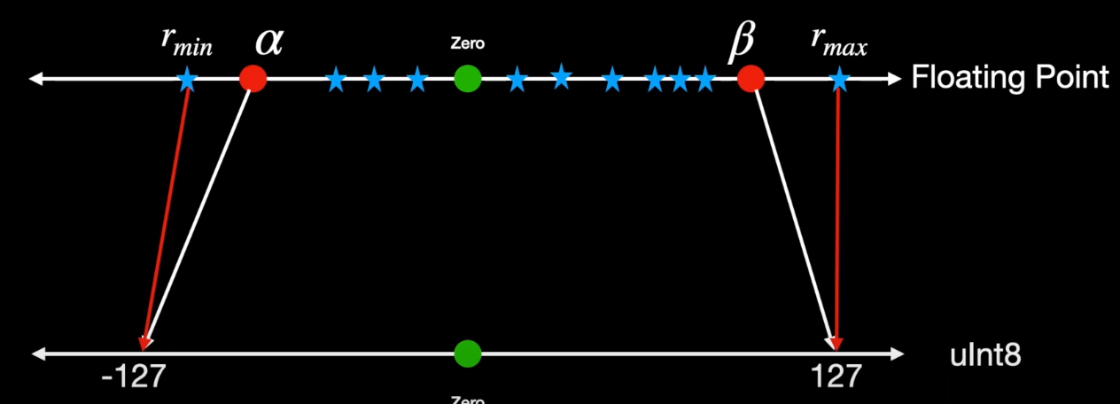
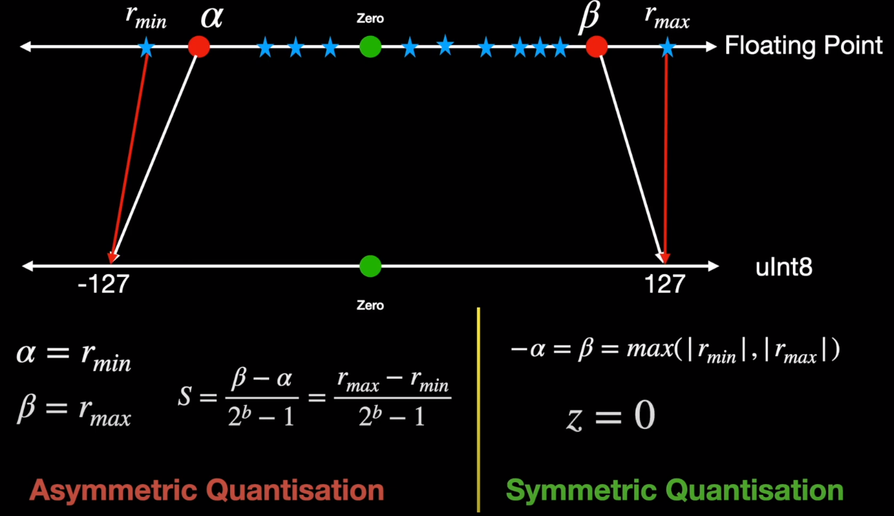
To learn how we can choose the scale factor and zero point, lets take an example input distributed like in the above figure in the real number axis. The scale factor essentially divides this entire range of the input right from the minimum value r_min to the maximium value r_max into uniform partitions. We can however choose to clip this input at some point say alpha for negative values and beta for positive values. Any value beyond alpha and beta is not meaningful because it maps to the same output as that of alpha. In this example its -127 and +127. The process of choosing these clipping values alpha and beta and hence the clipping range is called calibration.
In order to prevent excessive clipping, the easiest option could be setting alpha to be equal to r_min and beta to be equal to r_max . And we can happily calculate the scale factor S, using these r_min and r_max values . However, this may render the output to be asymmetric. For example, r_max in the input could be 1.5 but r_min could only be -1.2. So to contrain to the symmetric quantization , we need to set choose alpha and beta to be the max values of the two and of course set zero point to be 0.
Symmetric quantization is exactly what is used when quantizing neural network weights as the trained weights are already pre-computed during inference and it won’t change during inference . And computation is also simpler compared to asymmetric case as the zero point is set to 0.
Now lets take the example where the inputs are skewed to one direction, say to the positive side. This resembles the output of some of the most successful activation functions like ReLU or GeLU. On top of that, outputs of activations change with the input. For example, the output of actiovation functions is quite different when we show two image of a cat. So the question now is, “When do we calibrate the range for quantization?” Is it during training? Or during inference as and when we get the data for prediction?
Modes of quantization
So this question gives birth to different modes of quantisation based on when we calibrate the range. In Post Training Quantization or PTQ in short . We start with a pre-trained model without further training it. The only data needed from the model is the calibration data to calculate the clipping range and hence the scale factor S and zero point Z. This data in most cases comes from the model weights. Once we calibrate, we can then quantize the model and obtain the quantized model.
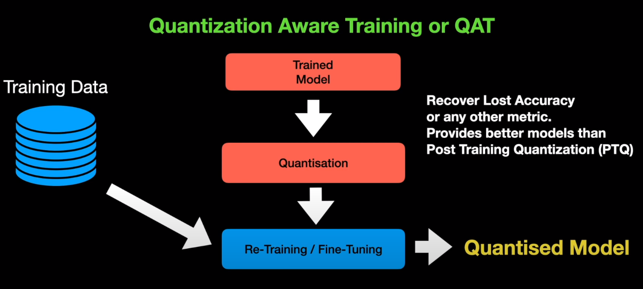
In Quantization Aware Training or QAT in short , we quantize the trained model using standard procedure but then do further fine-tuning or re-training , using fresh training data in order to obtain the quantized model. QAT is usually done to adjust the parameter of the model in order to recover the lost accuracy or any other metric we are concerned about during quantization. So, QAT tends to provide better models than the post training quantization.
In order to do fine-tuning, the model has to be differentiable. But quantization operation is non-differentiable. To overcome this, we use fake quantizers such as straight through estimators . During fine tuning these estimators estimate the error of quantization and the errors are combined along with the training error to fine-tune the model for better performance. During fine-tuning, the forward and backward pass are performed on the quanitzed model in floating point. But the parameters are quantized after each gradient update.
YouTube Video
Why not checkout the video explaning model quantization in deep learning
Summary
So that covers pretty much the basics of quantization. We started with the need for quantization, the different types of quantization such as symmetric and asymmetric. We also quickly learnt how we can go about choosing the quantization parameters namely the scale factor and zero point. And we ended with with different modes of quantization.
But how is it all implemented in PyTorch or TensorFlow? Thats for another day. I hope this video provided with some insight on Quantisation in Deep Learning.
I hope to see you in my next. Until then, take care!
